
1. Measurng money
2. Concepts
1. Depended variable - before interest bearin current were introduced
2. Independent variable
1. Scale variables - income versus wealth. income as a proxy for transactions. How to estimate wealth - firms and households, govn debt. Importance of expectations. Adaptive expectations - review by how wrong they were in the todays expectations. Yet-Yet-1=l(Yt-Yet-1) But you will make a systematic error, when data is trended. Rational expectations try to get rid of the systematic error. Aso people will use other data, other than previous income, to predicc current income.
2. Oportunity cost variables - returns on alternative assets, different interest
3. Own rate of return on money - implicit return on bank charges, inflation
4. Expectedinflation rate - adaptive expectations dont work again. Foward premium in exchange rates will capture rational expectations.
5. Other variables - real wage, riskiness of other assets, long run institutional changes
3. Identification and econometric problems - haard to define a demand curve. Scale variables etc. are not exogenously determined. Especially wealth and income. So we should use macro model instead of single Md model.
4. Conseptual problem - theory is predicting an optimum amount of money, but real world is different. Individuals very often adjust their money stock periodically. So we must include a theory of the adjustment to the optimum.
Rules out liquidity trap. Rules out significant relationship between interest rates and demand for money (rules out monetarists).
Expected inflation influences Md in hyperinlation. Recently they even think that even moderate inflation affects Md, that is why Md functions broke down in 1970s.
Demand for nominal balances is proportional to the price level.
Money multiplier
1. recognises that banks create money
2. retains a key role for authorities via control of monetary base (high powered money) and credit
Not all Banks use the same tools or operate in same institutional legal setting. Flow of funds identities impose conditions on monetary policy - fiscal position of the government and funding policies.
Buying and selling long and short term government debt. Primary determinant of monetary base - so high effect.
1. Dynamic OMO - intended to change the base money supply
2. Defencive OMO - ofset movements that could affect the monetary base
Central banks only managed government debt, but the Bank did buy some private investment in 1980's.
If the Bank wants to tighten the policy they SELL to
1. banks - substituting liquidity for long-term bonds. Money supply declines. No immediate effects on deposits
2. non-bank general public - multiplier fall in money supply as credit creation.
If govn uses OMO then interest becomes market determined and difficult to reconcile with funding policy.
Monetary base control never practised in the UK. Discussed in 83-4 and 90.
Richardian equivalence - if govn sells bonds then public saves more as expects future tax to rise and thi fset the sale os savings of bonds.
Unpopular, lowers base and direct effect on market rates. OMO makes interest rate policy effective. Overdraft system is hard to reconcile with monetary base control. Announcement effects are important.
Banks managed to overcome the corset by lending in overseas currency. They also guaranteed the firms bills - disintermediation. Rises uncertainty. Expensive to administer small exchanges.
1. Pre 1971 - direct control, credit ceilings
2. Competition and Credit Control 1971-3 - interes rates used
3. The Corset - targets for interest bearing elligible liabilities, penalties for too high deposits growth
4. Medium Term Financial Strategy 79-86 - targets for Ms, PSBR and interest used
5. Monetary Base Control never used
6. Overfunding 1980s - run down in banks' holding of government debt, cash shortages in the banking system were met by Bank acquisition of commercial bills.
7. Exchange rate mechanism - interest rates determined to maintain exchange rate.
Cost of capital - Change in Ms changes interest rate that changes investment and thus income.
We have to estimate the elasticities in this case.
FGF - feel good factor - between r and I.
LT - liquidity trap - between Ms and r.
Keynes believe in fiscal policy - IS is perfectly inelastic
Liquidity trap - changes in Ms cannot make r go below some r*.
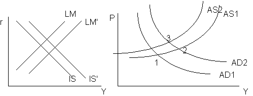
If there is unemployment, we might expect prices to fall. This is going to effect the LM curve. Real money supply increases - real balance effect. This effect is useless in liquidity trap.
Pigou effect - fall in the price level will influence the private sector wealth. This will increase the IS as spending will increase.
Fisher effect - Keynesians pointed out that in falling prices people will expect prices to fall even further and thus postpone their spending.
M-> spending. Demand for money is dominated by the transmission demand. Vertical LM curve. Increases in goverment spending will be crowded out 100%. But monetary shifts is inflationary, so LM curve increase will cause inflation that will shift the LM curve back. So the original equilibrium should be the long term equilibrium.
In reality, every shift in ISLM will probably lead to both price and income level changes.
Because both Pigou and real balance effect.

Because wages will rise because of inflation, the initial AD rise will lead to a decrease in AS.
So in real economics the differences arise from aggregate supply, not from AD and stuff like that. Money demand etc. in not very important.
1. Interest changes however have income effects that do not net out.
2. Availability of credit
3. expectation transmition
4. exchange rate