

The very simple case of Keynesian system can be extended to include govn. spending and tax. The assumption about govn. spending being exogenous is very bad. Usually G=gY g<0.
Flow of export is a function of exchange rate. Nominal exchange rate e=pound e/$ - the number of punds that a dollar can by. We are going to assume exchange rate is fixed - Bretton Woods system. System of exchange determination under IMF det up by Keynes. Exchange rate could only be altered if countries could show that they were running a BoP crisis.
So the flow of exports will be given. The leakage from the system take the form of imports - purchase of foreign goods. Imports are endogeneous and depend on GDP. Y=. Very important assumption is that the rate of interest is given. Monetary policy is accomondating - its aim is to stabilise exchange rate irrespective of the GDP.
Problem:everything is interconnected in Keynes.
Hicks:ISLM. Concentrated on
1. connections between S I Y and r
2. connections between Md Ms Y and r
Fix price assumption.
M(s&d)=kPY-br Y=M/kP+(b/kP)r if P and Ms constant Y depends on r.
r is the dependent variable and Y independent in the ISLM.
In ISLM rate can change because of real factors (I,S - monetarists thing) and monetary factors (Ms Md Keynes). But influence is indirect
The state of business confidence is given, so interest rate only determines:
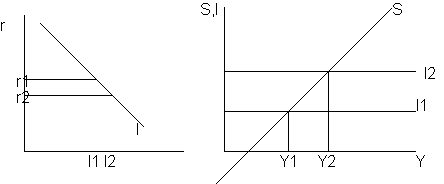
dY=dI/(1-c). So the level of income rises to Y2.
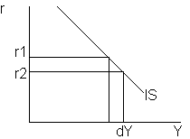
So the fall in the rate of interest increases Y.
Instead of asking what would happen to income we ask - what would happen to the interest if income rises.
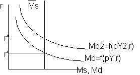
Md=f(pY,r). If the level of Y rises the Md will also rise. This happens very rappidly as financial markets move rapidly. Infinite pair of Y and r defines an LM curve:
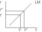
L=M (demand for money= supply of money) is the LM curve and depicts the monetary equilibrium. So we have 2 curves, an upward and a vertical:
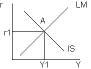
General incme expenditure equilibrium. It is very good for analysing the different effects of fiscal policy and the monetary policy.
We assume that it takes the form of increased G. They are not autonomous, but decided. This in macro level is comparable to increase in I:
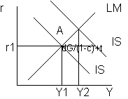
Y does not rise by the same amount. Increase in G tends to rise Y, but this rises the Md, this leads to a rise in r. So Y rises, but not by the same amount as the multiplier dG/(1-c)+t suggerst because of the crowding out of the private investment. The extent of crowding out depends on the slope if LM curve. If LM is vertical, crowding out=100%, if the LM is horisontal, there will be no crowding out(liquidity trap, absolute liquidity prefference).
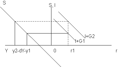
Y is increased by dY=1/(1+c)+t.
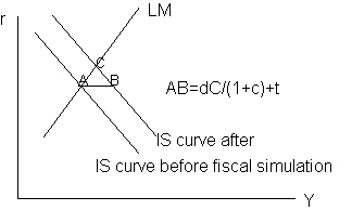
This does not take account the pressure on interest caused by the raise in Y. So you move after ab to C. Because the investment decision is interets rate sensitive. The fall in investment is less than the rise in dG, so crowding out is less that 100%. If no liquidity prefference LM is vertical, dG=-dI. In that case there is no point in relying on fiscal policy.
What causes the shifts (system out of equilibrium).
The LM curve tells you what the rate of interest will actually be. If we are left below IS curve the I>S. This will lead to an income starting to rise. The demand for money starts to rise. So we treck up our LM curve. The economy can be off the LM curve on very short time as financial markets react very quickly.
Very simplistic view:
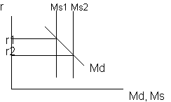
Not correct to say that the Ms increase will lead to reduction in the rate of interest. The reduction in r leads to increase in Ms.
Fall in r leads to increase in interest, rise in income, rise in the demand for money. So this picture is incomplete, for complete picture we have to refer to ISLM.
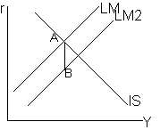
At point B investment exceeds savingsa and Y rises and nominal demand for money rises. So rate of r settles between AB.
It is often assumed that monetary and fiscal policies are independant. It was not the case until 1979. Primary place was for fiscal policy until 1970 and monetary had a supportive role, it was accomondating. Suppose economy was in recession and govn wants to help. So it shifts IS curve up and interest rates rise. If monetary authorities react to keep r at a target. Violent fluctuations were regarded as undesirable. So money supply must increase to prevent deviations:
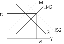
So the supply of money becomes endogeneous to countereffect the crowding out of private investment.
Highly centralised collective bargaining is not common bargaining, but fragmented monopolies.
When e rises, so do P, W and P again.
Leap-frogging cost-push inflation. There is a fair set of wage differentials. This fairness has been a claim reason for trade unions. So if one industry has excess demand, the wages there would rise. Now other people want a pay increase too. Again the level of aggregate demand has got nothing to do with it.
No point in adopting a tight fiscal policy when you have a cost-push inflation. Incomes policies should work. Tax should punish too soft employers.
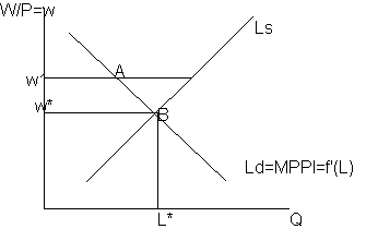
In a free market the forces of competition will ensure that the wage will fall to w*. Keynes rejected that the w could fall even in a big excess of Ls, even in a competitive market. If there is an excess suplly then money wage would fall, Pigou took it for granted that the real wage would fall as well. Keynes did not accept that. Keynes thought that Pigou might have linked Ms to P, then link would be valid. W/P=MMPl, arranging P=W/MPPl=MC in perfect competition.
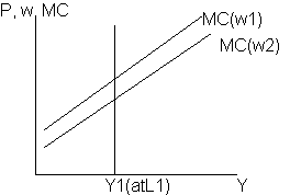
MC depend on the level of money wages. The slope of it depends on MPP. So a decline in money wages will cause an equiproportional change in price. So the real wage will not fall if there is unemployment. It is a thing of balanced deflation.
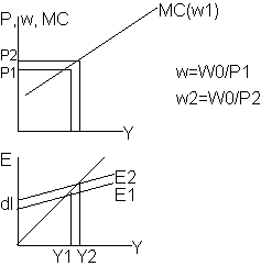
SIMPLIFYING assumption is that the money wage rate remains the same. Can be relaxed, but then MC cannot be determined.If Ls>Ld, then if I rises, E rises, Y rises, MC(w0) rises, prices rise and real wage rate goes down. Alterations in the money wage does not alter real wage.
Imports are endogenous as firms demand more imports. Exports are exogeneous depend on foreign investors. This is a great oversimplification. Exports are det. by exchange rate that is given, but govn spending varies with income.
Next week: does a fall in W and P influence E?