

Model that is free standing, but not very in one place
a. Theory of output and employment
We assume a given short run production function. Capital stock is given. Techonogical knowledge is given
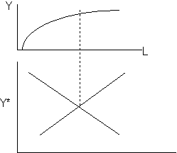
Supply and demand have assumption that substitution effects dominates income effect. Demand for labour is MPP of labour.
Pigou says the unemployed would compete with employers to make the labour market clear.
b. What determines the rate of interest
Marshal and Fisher tried to find out.
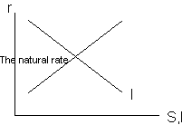
No widthdraws from the system. When I falls, C will rise.
c. The quantity theory of money.
Previous 2 were real compartments of economy. What determines the absolute price level and nominal wage rate. Supply of money determines inflation. Incoome version of Fisher's equation allows Classical theory to be compared with Keynes' one.
MV=PY, ML=kPY k-how much income you are willing to hold in money form. When in equilibrium ML=MS, so M=kPY. Everything but P is constant. P is bought about by Cash Balance system.
Arguead against 1.b. When I falls, the C will not rise and Y will fall. Through multiplier effect. If r is given, so is I. Saving is not and depends on Y.
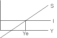
Here income declines when I declines. Ye=(-a+I)/(1-c)
Include government. I+G=T(f(Y))+S, then Ye=(-a+I+G)/(1-c+t)
Include Open economy. Nominal exchange rate e is given. Ignore capital flows. X=f(e,world trade), so X is exog. M=f(e,Y). Ye=(-a+I+G+X)/(1-c+t+m)
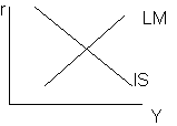
Fall in interest leads to rise in investment and income. Income leads to increase in savings. IS curve can shift by
a. rise in a - autonomous consumption
b. animal spirits (I rises)
c. Fiscal policy - rise in G, fall in T
d. Increase in exports
LM is controlled by government. It is controlled by demand factors. Ms becomes endogenous.
a. Monetary and fiscal policy
Expansionary fiscal policy - partial crowding out. If you use monetary policy as well, you would increase Ms. Then no crowding out. Accomondating monetary policies. Now Ms is endogeneous - to stabilise r.
ISLM models are assuming stable prices.
But effects of money wage and prices start to fall can be analysed:
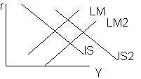
Ms remains 0, but price level fall will shift LM. This will put pressure on interest rates and increases investment. Then Pigou (real balance effect). Real value of private wealth will rise. This will stimulate consumption and shift IS curve to IS2.
Inflation - excess of aggregate demand. Y* is the national income limit. There is no guarantee that E=Y*
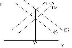
When IS increases for somehow LM shifts northwest because as prices rise, real stock of money is reduced. When real Ms will not fall (monetary accomondation) then Ms groth and inflation should be similar. However, monetarist interpretation is that Ms growth causes inflation. In this case Ms is caused by inflation.
Friedman- "Inflation is alwayss nd everywhere a monetary phenomenon". Friedman meant that inflation was caused by excessive rate of growth of Ms - monetary mismanagement. One example is when Ms growth exceeds real income growth (political influences). Keynes said that Ms is no importance itself, it only matters when Ms alterations produce alterations in rate of interest and thus changes in Y.
The other assumption was that real economy is selfadjusting (ie of the independence of Bank of England). Real sector is unaffected by monetary one (except in the short run).
1. Leap frogging (claims are based on comparability)
2. class strugle (workers and capital fight for the share of GDP)
3. real wage resistance (workers become acustomed to W/P). If for some reason it changes then workers can only affect W and they will. Wage price spirals occur. You assume that monetary policy is accomondating.
4. NAIRU models. It needs not to corresponf to full employment
ABS(Ex+Em)>1
This can only be interpretated as a demand for imports and epports when Sx=Sm=infinity.
Devaluation is an expenditure switching policy
Xup Mdown, Injections up, income up, imports up.
If an expenditure switching policy is succesful it must be accompanied by expenditure reducing policies. Otherwise demand pull inflation will ensure. This inflationary gap will reverse the depreciation. In 1950-s we had very low unemployment. That isnot true when economy starts of with underemployment.