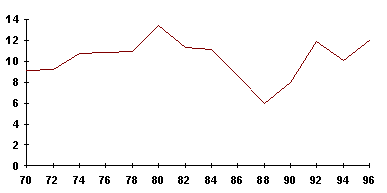

Savings ratio(SR) is the average propensity to save, SR = Personal Disposable Income(PDI)/Savings(S). SR has fluctuated widely since 70-s being between 14% and 4%. But as PDI = Consumption(C) + S we can analyse the movements and theory based on C and PDI. Furthermore taxes can be seen as exogenous, so PDI can be approximated to Y. Latter on when I reach my conclusion I will return to APS. When specific numeric values are used they have been optimised for APS to include years 1950-90, and although the factors influencing APS have remained mainly the same these figures are approximate and a better fit could be obtained if date is optimised for 1970-96, because some things (like housing) have changed in importance. Savings ratio looked like:

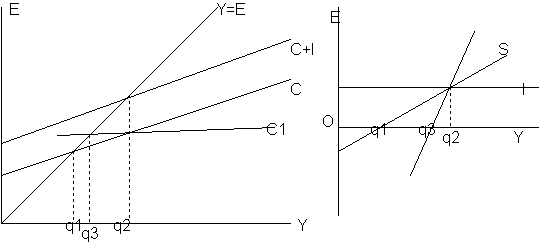
Keynes classical theory was that C=A+MPCxY or Y=C+S, where A is a constant called autonomous consumption and MPC is the marginal propensity to consume. This equation implies that savings is a type of super good that can be substituted for consumption. By diagram:

E is expenditure in here and I investment.
As seen the movement in savings ratio can occur because of a change in income that will cause movement along C curve and thus cause relatively more savings. Or it can be because of a shift in C curve, caused by, as Keynes suggested, capital gains etc. Keynes model is also thought to work in short-run, and here comes the major difference between the Keynes and the Rational expectations(RE) view. According to RE, in the long run one could have something like this Keynes model, as people's expectations of their future permanent (or life cycle in the case of Modigliani) will change, but in the short-run, in which Keynes was interested in as well, consumption will look more or less like C1 and thus savings like S1. Furthermore, the consumption function will shift around based on expectations of inflation, house prices, previous income etc.
To prove all that we must make first of all a minor adjustment. The correlation between actual APS and predicted one is better when C is put to the logarithmic form - i.e. C=AYb where b is the elasticity of consumption, denoting c=log(C) and y=log(Y) we get c=k+by, where k is again a constant. Putting values in:
C=3.65+0.89Y
c=0.19+0.95y
This function can explain the general trends in savings ratio up to 1980-s. But it cannot predict the fall in savings ration from 1980-s. Furthermore writers have said it is wrong to count savings as a good, that the savings are used to even out fluctuations in income. This view is called the life cycle hypothesis by Modigliani (or with similar outcome permanent income hypothesis by Friedman). Graphically:
|
|
Dissaving Saving |
Permanent income depends on the expectations of the previous incomes. For example if people base their expectations of next income on 3 previous time periods(3 can be any number) then:
yp=(yt+y(t-1)+y(t-2))/3
ct=0.27+0.94yp
This equation looks very much like the equation above, elasticity being only 0.01 smaller. But there is a very important difference here - the short term(one year) elasticity is only 0.31. That means when the income were to rise by 10% then the consumption would go up approx. 3.1% on the three subsequent years not all on the first year. That gives rise to a substantial savings in the first two years. This equation can estimate the consumption more accurately. But people will not value the previous information evenly - information a while ago is less important. So it is right to include geometrical weights to expectations:
ypt=(1-w)yt+w(1-w)y(t-1) +w2(1-w)y(t-2) ...
1>w>0
ct=kyt+et e is the error, so is k
summing the GP ct=k(1-w)ypt+wct-1
That means current consumption is based on the previous consumption and the expected income this year. Putting in numbers:
ct=0.26ypt+0.73ct-1+0.05
Income is predicted by rational consumers with all the information they have - i.e. the information that they know in t-1 period and new uncorrelated information that becomes available in t. Under permanent life time hypothesis they will try to even out the cycles in consumption. So in equation
ct=kct-1+et
the et term is the error and with mean 0 and uncorrelated with any of the variables in the equation. This is Euler's equation and suggests that consumption could not be predicted. When k=1 the situation is called a random walk as the ct can either go up or down. However the evidence suggests that k>1 because income rises over the time and people expect it to rise. Furthermore et seems to be correlated with itself and thus the random walk model could be enhanced. This last equation was used a lot a while ago and called adaptive expectations. But the consumers will have a permanent bias when income changes regularly. RE dealt with that including more variables, that I introduce later, to consumption function. Also it has been suggested the consumers have a target long-term income. In short term there are shocks affecting consumers, so they will try to balance the current consumption to meet his long-term target. This is called the error correction method and it says that the correlation is between the change in ct and yt not in the absolute values.
ct=a+bypt+gst-1+ft
In here s is the savings ratio in the period before (i.e. people learn from their previous experience of e). denotes inflation, that is also thought to be one of the major causes of change in APS. It reduces the real value of debt. So originally it was thought by Keynesians that higher levels of inflation reduced savings and forced people to consume more as the value of savings fell. But after 1970 the theory was changed. Consumers are largely net creditors. So inflation is like a tax on their savings to the government who is a net debtor. This tax is not included in the PDI. Although in long-term the effect could 0 due to lower taxes arising from reduced national debt, in the short term savings will rise. Also there is usually a lag between receiving income and spending it, with high inflation this will decrease consumption. People also hold some money as a proportion of their wealth for rainy days. With inflation its real value falls so people have to make it up by saving more. Businesses are also included in the consumption. Their stock (which is savings)appreciates, so they save more. Inflation also favours young, who borrow to buy their house. As house is a saving it will again rise APS. So inflation was the major cause for the rise in savings in 1970s.
House prices are another major item affecting APS. The evidence is more of an empirical sort here. Economists tried to find explanation for the rise in APS in late 80s. Credit liberalisation and the reduction in the uncertainty of income (i.e. the income growth stayed more stable) were also playing their part. One can have a theoretical reasoning that says when house prices went up people could either sell their houses and use the money to spend quite a lot or they could borrow more on existing housing with the liberal credit policy. This all increased consumption. House is a part of wealth and people's wealth increased. This is generally attributed as being a source of more consumption as people's expectations were not set for higher wealth and they find they can allow themselves a lot more without affecting their life cycle hypothesis. SO the equation would look like:
C=0.06Wt+0.7Yt
where W is wealth at time t. This equation could be again extended to delta c form.
The rise in house prices also attributed for the reduction in APS in 72-3 and late 80s and its fall made the savings to rise again in 1990s. High levels of savings in 1990s were also due to larger uncertainty, due to recession, and high interest rates originally thought to have no effect. Interest rates are also strange because theoretical reasoning for them affecting the savings can be put either way and in practice there was very little correlation before 1989. Although there was some lagged correlation (as seen from the graph) and much more correlation in 1990-s - high interest was causing savings.
People also saved more for precautionary purposes in 1990s. As the house prices have started to rise rapidly again, the savings ratio should fall soon. The self-sustained growth and low inflation should mean the same. Credit availability have also been reduced by stricter banking regulation after Barings collapse and partially also with higher interest rates, so people cannot borrow so easily and thus have consumed less during 90-s.
So the finial equation with values in it includes a provision for the change in house prices(RHP) and uncertainty():
ct=a+bypt+gst-1+ft+hRHP+k
ct=-0.009+0.73ypt+0.19st-1-0.09(*-t)+0.018RHP-0.51
This equation allows the prediction of the savings ratio to quite a large extent. In calculating the prediction we must take the contribution of each individual item relatively. That means, for example, that when the average inflation (*)over a period of time was 5% and this year we have 6% then the actual contribution is 1% and we should use that for our figures. So *=5% in that example. However we have not included the split between consumer durables and other current goods in here. Economist have said these are so different and the motives for buying them are different as well, so there should not be just one c. No study has yet proved any significant relationship, though. There should be internal substitution occurring between investment and consumption when interest rates rise, but no study has yet shown that this holds true. Same applies to the constrain on loaning in crises hypothesis, that predicts that the consumption can move down but cannot move up for families with liquidity problems as they cannot get credit freely.
Now as y appeared in the equation all the factors that influence y influence also c. That means that unemployment affects the savings ratio and so do world influences and trade cycles. Also demographic changes will change people's lifetime hypothesis - when they will expect to live longer and be longer pensioners then they will save more. But these effects are very long-term ones and thus cannot be very relevant to this 25year period. Similarly institutional and social changes influence savings. For example the appearance of well established pension funds caused savings to rise in the 70s. That can explain why savings are high now. Different groups of people have also different transitionary incomes (deviations from the lifetime income) so they are expected to save more. One example with high transitory income are farmers, so when their proportion rises, so should savings.
Richer people, especially those in top 20% , also save more as bequests. Rising income inequality from 1979 onwards could attribute partially to the rise in savings ratio. This means savings is a luxury.