
Custom Search
1)
Introduction
a) Common expression is export led growth
b) However, once countries start growing, imports will increase.
c) Lately BoP crises in several countries, followed by slower growth.
2)
Theory
a) Keynesian theory of Y=C+I+G+(X-M).
b) Injections will have multiplier effect on GDP.
c) Increase in X is an injection.
d) However, M depends on GDP, while X does not.
e) Thus for countries to continue on growing, something must balance M.
f) Explain how BoP deficit will lead to currency devaluation, financial instability, raise in interest rates, reduction in investment and GDP.
3)
Data
a) Cross sectional data from international economics handbook
b) Plot first and look for lags
c) Correlate exports and GDP growth (real terms). Unlikely anything.
d) Now correlate balance of payments (X-M) and GDP growth. Likely lagged correlation.
e) Do (GDP)’=c+X-M and do formal tests as to whether X is significant. Look at R2 values. Use data for cross country pooled estimates as well (Average growth of exports over past 30 year and average growth in GDP).
f) Discuss whether change in exports more appropriate than absolute, and same with GDP. Look at loglinear model instead of linear.
4)
Analysis
a) Other factors influencing GDP, like interest rates, world economy, unemployment, technological shocks (oil price).
b) Large measurement errors.
c) Not very good idea to pool data because normality of errors etc.
5)
Conclusions
a) Economies getting more open, so in general export rises. But it is the relative magnitude of exports to imports that matters.
Price level AS

![]() For the economy as an
aggregate, in a simple model, everything that is produced is also consumed. And
only things are produced that have demand. Thus aggregate demand and supply are
the same things. However, when one takes stock accumulation into account, then
the separation of AD and AS is possible. Although no-one has ever proven the
relationship empirically it is thought that the AD and AS curves behave just
similarly to normal D and S curves, and the economy is where they intersect.
For the economy as an
aggregate, in a simple model, everything that is produced is also consumed. And
only things are produced that have demand. Thus aggregate demand and supply are
the same things. However, when one takes stock accumulation into account, then
the separation of AD and AS is possible. Although no-one has ever proven the
relationship empirically it is thought that the AD and AS curves behave just
similarly to normal D and S curves, and the economy is where they intersect.

![]()
However, when one of the curves changes, then initially price level will remain the same and stocks will be either depleted or increased, and economy will be in temporarily out of equilibrium. This cannot last forever, and thus concepts of cost-push and demand-pull inflation are introduced. They essentially describe why one curve (AS in case of cost push and AD in case of demand pull) will cause the new equilibrium to be at higher price level, thus causing inflation. In real life there is always some inflation present and there are inflationary expectations, so empirically I will have to test the temporary increase in inflation. Also, sometimes GDP can rise instead of price, especially when there is spare capacity. Thus the test I will do will show the effects as to whether it is the price level or the GDP that will change after cost-pushes or demand pulls. For example, cost push can be explained by the increased costs of production at each output level, meaning the shift of AS curve to the left. This will be accompanied by a greater payment to the factors of production, eventually increasing their ability to consume and thus AD.
Price level p2 p1
![]()
As seen the new output is the same, but price level is different. It is cost push, because Y* is initially pushed inwards. Similarly demand pull inflation occurs when AD curve shifts out first, causing firms to produce more than optimal and thus making them increase their price. Thus the empirical testing will involve mainly determining which lags occur first: will it be the AD that normally shifts out first, or will it be the AS that contracts first.
Cost push inflation can be empirically best analysed by looking at the payments to the factors of production. Cost push inflation occurs when real wage increases (payment for labour); input prices or raw material prices increase (land payment, this will also include oil price shocks and real exchange rate changes); interest rate changes (payment for capital); or the profit margins get larger (entrepreneurship payment, includes the increase in the monopoly power).
Demand pull inflation on the other hand can occur because of the sudden changes in peoples wants. This is normally associated to Keynes and is really quite hard to gasp intellectually. However, empirically the demand pull inflation is occurring when the GDP increase will precede the price increase (from AS AD diagram). The aggregate demand can increase without the accompanying increase in productivity (i.e. without the payments for the factors of production increasing) due to numerous factors. In classical theory where GDP=MV=PT, the change in money supply will increase GDP and thus price level, when the velocity of money is constant. In a more Keynesian framework the reduction in savings rate (or increase in consumption) will lead to increased demand. Also when government policies and spending increases, the AD will increase. The inflation is a domestic phenomenon; thus one must take the changes in import penetration (assuming Marshall Leaner condition holds) into account. Similarly the demand for domestic goods will be changed by the change in the real effective exchange rate.
Statistical
analysis.
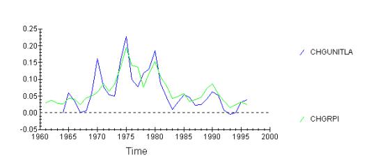
Let me take the variables first one by one. Starting from
labour and unit labour costs, looking at the relationship between the unit
labour costs and the RPI, first looking at absolute relationship, and then the
relationship between changes in the variables:
As seen, labour costs are growing slower than the RPI, and there is significant correlation between the changes in UL costs (ult-ult-1)/ult and changes in RPI. Furthermore, the changes in UL tended to precede changes in RPI until 1980-s, and after that they lagged behind. This suggests that cost-push measures operated until 1980-s and after that demand-pull measures set in. I will leave the OLS analysis later, so I can include all the variables affecting RPI, because omitting variables would make my OLS biased.
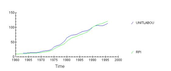
Turning now the attention to second factor of production, land, I will examine the relationship between raw material prices and RPI.
It is clear from this graph that the raw material prices
started growing much earlier in 1970-s than the RPI, pulling RPI along. this of
course is due to the two oil price shocks that increased the price of raw
materials sharply. However, after 1985 the raw materials ceased to become more
expensive, while the RPI continued to grow. This growth is then likely to be
associated with factors other than cost-push.
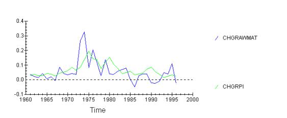
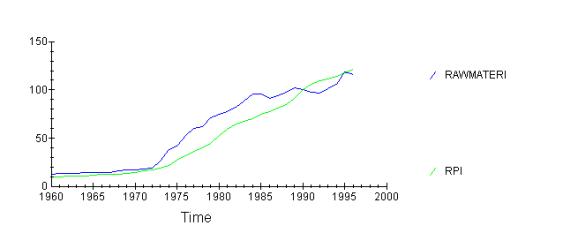
Again, the oil price shock of 1974 is very clear, however,
prices will rise after two years. Raw material prices clearly precede RPI by 2
years, however, the recent increase of 1994 has not had a significant impact.
That might be because government’s strict policy of keeping inflation under
control, or due to high unemployment, implying that the real wage is too high,
and thus is more important than the raw material costs. Also the tertiary sectors
of economy and services are now more important. They use very few raw
materials.
Thirdly let me look at the price of capital, the interest rate.
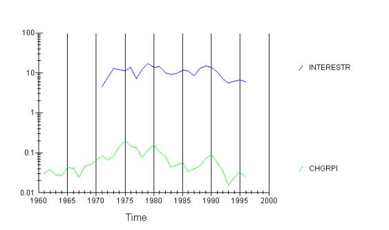
Again, it is clear that the interest rate movements preceded
RPI movements. However, there are probably numerous factors, like government
policy, exchange rate, etc., that affect both interest rate and RPI. Thus this
correlation is not very meaningful a priori. Still, the interest rate cuts in
1990s probably helped to bring the RPI down.
There is unfortunately no measure for the entrepreneurship, although when firms want to increase their profit margins, maybe because their have market power increases or due to cartel agreements, then inflation should occur.
Now how much of inflation can cost-push measures explain? Doing a simple OLS without lags:
Dependent variable is CHGRPI
26 observations used for estimation from 1971 to 1996
Regressor Coefficient Standard Error T-Ratio[Prob]
INTERESTR .8882E-3 .0012895 .68877[.498]
C .017275 .012417 1.3912[.178]
CHGUNITLA .65457 .079189 8.2659[.000]
CHGRAWMAT .10019 .046711 2.1449[.043]
*******************************************************************************
R-Squared .85075 R-Bar-Squared .83040
S.E. of Regression .019217 F-stat. F( 3, 22) 41.8006[.000]
Mean of Dependent Variable .076737 S.D. of Dependent Variable .046661
Residual Sum of Squares .0081241 Equation Log-likelihood 68.0309
Akaike Info. Criterion 64.0309 Schwarz Bayesian Criterion 61.5147
DW-statistic 1.5970
*******************************************************************************
* A:Serial Correlation*CHSQ( 1)= .79637[.372]*F( 1, 21)= .66354[.424]*
* B:Functional Form *CHSQ( 1)= 1.3774[.241]*F( 1, 21)= 1.1748[.291]*
* C:Normality *CHSQ( 2)= 2.1978[.333]* Not applicable *
* D:Heteroscedasticity*CHSQ( 1)= .53681[.464]*F( 1, 24)= .50597[.484]*
There are no problems with the data (heteroscedacity etc.). Interest rate is not significant at 5% level, and the constant is neither, but other factors are. R2 is above 0.8 indicating a good fit.
Let me now look at the demand pull indicators. First the changes in MS.
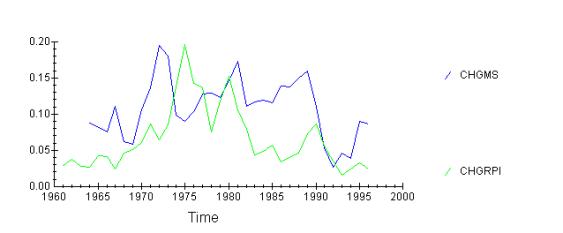
As seen, MS quite strongly precedes the RPI, in 1970-s by 4
years, however, after 1980 the lag disappears. There were numerous financial
innovations occurring during 1980-s together with financial liberation. That
meant that the money supply increased considerably, but inflation did not
follow.
Secondly I want to look at consumption.
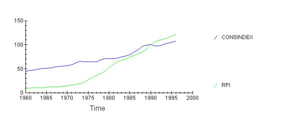
As seen consumption rises slower than the prices. However, it
is also clear that at the end of 1980-s consumption suddenly rose, and the
prices followed 2 years later. Similarly in 1990 consumption fell and prices
stagnated a year later. This presents a strong evidence in favour of demand
pull theory.
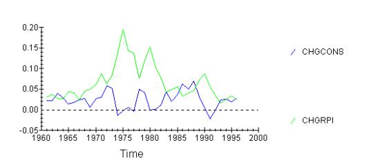
As seen, consumption changes will precede inflation changes by
two years.
Secondly I want to look at the PSBR.
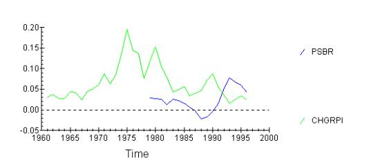
There is very little relation. This can be because PSBR is
very politically targeted variable. Also both of the variables are affected by
the business cycle. Anyway, this diagram suggests that PSBR and RPI are
inversely related, meaning higher borrowing will lead to lower inflation. This
is not what demand-pull inflation suggests. However, it might be reasonable
when one thinks of the interest rising after increase in PSBR. This will lead
to a reduction in economic activity and thus less inflation. However, when one
looks at the government consumption directly:
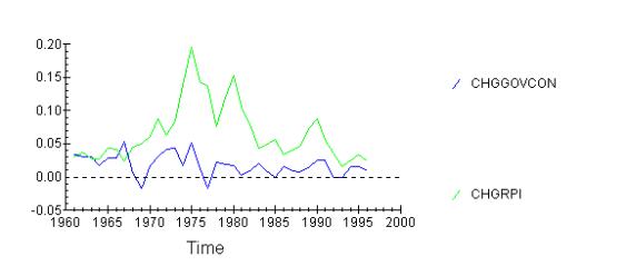
There appears to be some correlation. However, the lag
structure is unclear, possibly because inflation will adjust government
consumption plans (due to increased taxes etc) accordingly. Still a 2 yeaar lag
is not unreasonable.
Lastly I would like to look at the GDP itself. When the increase in GDP precedes that of RPI, it suggests demand-pull inflation.
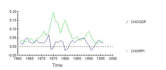
This shows how increasing GDP will cause inflation after a
year. And high inflation in turn forces government to step in and cool off
economy, leading to reduction in GDP. One should notice that both consumption
and GDP will have lags of similar magnitude. They are also longer than the lags
for cost-push factors, suggesting that it takes longer for the demand increases
to work themselves to the prices, because they will have to go through the
market mechanism. Factor cost increases will be incorporated to the price
levels by firms much quicker.
Let me now formalise the argument and do an OLS test with 2 year lags. I will not use PSBR because PSBR and government consumption are likely in multicollinearity.
Dependent variable is CHGRPI
29 observations used for estimation from 1967 to 1995
*******************************************************************************
Regressor Coefficient Standard Error T-Ratio[Prob]
C .018161 .025827 .70320[.489]
CHGMS .30809 .20824 1.4795[.152]
CHGCONS(-2) -.32178 .64160 -.50153[.621]
CHGGOVCON(-2) .93240 .49305 1.8911[.071]
CHGGDP(-2) .65861 .68860 .95644[.348]
*******************************************************************************
R-Squared .22663 R-Bar-Squared .097735
S.E. of Regression .042525 F-stat. F( 4, 24) 1.7582[.170]
Mean of Dependent Variable .074240 S.D. of Dependent Variable .044769
Residual Sum of Squares .043401 Equation Log-likelihood 53.1669
Akaike Info. Criterion 48.1669 Schwarz Bayesian Criterion 44.7487
DW-statistic .77389
*******************************************************************************
* A:Serial Correlation*CHSQ( 1)= 11.9058[.001]*F( 1, 23)= 16.0191[.001]*
* B:Functional Form *CHSQ( 1)= 1.4790[.224]*F( 1, 23)= 1.2361[.278]*
* C:Normality *CHSQ( 2)= 2.3279[.312]* Not applicable *
* D:Heteroscedasticity*CHSQ( 1)= 2.7639[.096]*F( 1, 27)= 2.8444[.103]*
This is not a good regression. First there is serial correlation present, secondly none of the coefficients is significant and lastly consumption is with wrong sign. It is probably so because I included GDP - this is highly correlated with other measures. Leaving GDP out,
Dependent variable is CHGRPI
29 observations used for estimation from 1967 to 1995
*******************************************************************************
Regressor Coefficient Standard Error T-Ratio[Prob]
C .021502 .025546 .84170[.408]
CHGMS .30749 .20789 1.4791[.152]
CHGCONS(-2) .18360 .36331 .50535[.618]
CHGGOVCON(-2) .83982 .48263 1.7401[.094]
*******************************************************************************
R-Squared .19715 R-Bar-Squared .10081
S.E. of Regression .042453 F-stat. F( 3, 25) 2.0464[.133]
Mean of Dependent Variable .074240 S.D. of Dependent Variable .044769
Residual Sum of Squares .045056 Equation Log-likelihood 52.6245
Akaike Info. Criterion 48.6245 Schwarz Bayesian Criterion 45.8899
DW-statistic .75639
* A:Serial Correlation*CHSQ( 1)= 12.6615[.000]*F( 1, 24)= 18.5989[.000]*
* B:Functional Form *CHSQ( 1)= .89113[.345]*F( 1, 24)= .76087[.392]*
* C:Normality *CHSQ( 2)= 4.0890[.129]* Not applicable *
* D:Heteroscedasticity*CHSQ( 1)= .64054[.424]*F( 1, 27)= .60984[.442]*
Now the consumption is with the right sign, but it is still not significant. And ther is serial correlation present. That means there must be an inherent flaw in my analysis. Doing the regression without lags:
Dependent variable is CHGRPI
29 observations used for estimation from 1967 to 1995
*******************************************************************************
Regressor Coefficient Standard Error T-Ratio[Prob]
C .030527 .017948 1.7009[.101]
CHGMS .63349 .17542 3.6113[.001]
CHGCONS -1.3976 .29893 -4.6753[.000]
CHGGOVCON .33743 .38573 .87478[.390]
*******************************************************************************
R-Squared .51064 R-Bar-Squared .45192
S.E. of Regression .033144 F-stat. F( 3, 25) 8.6959[.000]
Mean of Dependent Variable .074240 S.D. of Dependent Variable .044769
Residual Sum of Squares .027462 Equation Log-likelihood 59.8031
* A:Serial Correlation*CHSQ( 1)= 6.4353[.011]*F( 1, 24)= 6.8446[.015]*
* B:Functional Form *CHSQ( 1)= .35479[.551]*F( 1, 24)= .29726[.591]*
* C:Normality *CHSQ( 2)= 3.0858[.214]* Not applicable *
* D:Heteroscedasticity*CHSQ( 1)= 2.3016[.129]*F( 1, 27)= 2.3276[.139]*
Now the coefficients are significant, but the consumption has a wrong sign and there is still serial correlation. I could go into autoregressive models, but I clearly have no data on the avtual lag structure. The fact that consumption is with another sign suggests that increased consumption initially increases output and stops inflation. I think that the causation is the other way round - when inflation is higher people tend to save more for rainy days and consume less, because the real value of their wealth and savings are eroded. That is why the wrong negative effect. However, the inflation does depend very heavily on monetary factors.
In conclusion, it seems that two factors from both cost-push and demand-pull inflation are significant - unit labour costs, raw materials and money supply and consumption. I will combine them in a single equation together with government consumption and interest rate and then without the last two, to do an F-test in order to asses whether I can safely exclude them:
Dependent variable is CHGRPI
25 observations used for estimation from 1971 to 1995
*******************************************************************************
Regressor Coefficient Standard Error T-Ratio[Prob]
C .019143 .012548 1.5257[.144]
CHGMS .24573 .10668 2.3035[.033]
CHGCONS -.51727 .18802 -2.7512[.013]
CHGUNITLA .57963 .086002 6.7397[.000]
CHGRAWMAT .075853 .040946 1.8525[.080]
INTERESTR .1164E-3 .0012350 .094224[.926]
CHGGOVCON -.15262 .26107 -.58458[.566]
*******************************************************************************
R-Squared .90580 R-Bar-Squared .87441
S.E. of Regression .016422 F-stat. F( 6, 18) 28.8484[.000]
Mean of Dependent Variable .078848 S.D. of Dependent Variable .046338
Residual Sum of Squares .0048543 Equation Log-likelihood 71.3612
Dependent variable is CHGRPI
29 observations used for estimation from 1967 to 1995
*******************************************************************************
Regressor Coefficient Standard Error T-Ratio[Prob]
C .016944 .010396 1.6299[.116]
CHGMS .31329 .10810 2.8980[.008]
CHGCONS -.66035 .19628 -3.3644[.003]
CHGUNITLA .46470 .071609 6.4894[.000]
CHGRAWMAT .10440 .045621 2.2884[.031]
*******************************************************************************
R-Squared .84769 R-Bar-Squared .82230
S.E. of Regression .018872 F-stat. F( 4, 24) 33.3930[.000]
Mean of Dependent Variable .074240 S.D. of Dependent Variable .044769
Residual Sum of Squares .0085477 Equation Log-likelihood 76.7270
Akaike Info. Criterion 71.7270 Schwarz Bayesian Criterion 68.3087
DW-statistic 1.9077
* A:Serial Correlation*CHSQ( 1)= .2913E-4[.996]*F( 1, 23)= .2310E-4[.996]*
* B:Functional Form *CHSQ( 1)= .35135[.553]*F( 1, 23)= .28207[.600]*
* C:Normality *CHSQ( 2)= 1.8841[.390]* Not applicable *
* D:Heteroscedasticity*CHSQ( 1)= 6.4664[.011]*F( 1, 27)= 7.7481[.010]*
Ho: government consumption and interest rate are insignificant
H1: they are significant
Doing an f-test, F=(RSSr-RSSur)(n-k)/RSSur
|
F critical 1,17
5%=4.75 |
||
|
F= |
12.9344 |
>critical |
|
reject H0 |
|
|
thus my unrestricted model is still better. This is due to multicollinearity.
To test whether the inclusion of demand-pull variables was significant let me do the f-test to compare cost push and demand-pull added:
H0:cost push is sufficient
H1:it is not.
|
F critical 1,21
5%=4.35 |
||
|
F= |
14.1453 |
>critical |
|
reject H0 |
|
|
Thus it is better to include demand-pull variables as well.
As seen, both demand pull and cost-push variables are significant. However, demand-pull variables are harder to pinpoint and they also have lower effect than cost-push. From the graphs it can be deduced that at some periods cost push factors might have been more important than in the others. Unfortunately my statistical skills do not allow me to analyse so complex relationships. It is also evident that the multicollinearity was present. Taking cross-sectional data of several countries would solve that.