
Custom Search
Investment is thought of as the essential determinant of long-run growth and economic cycles. In this essay, I will describe the different forms of investment, look at the behaviour of investment in the UK, and try to explain its behaviour by using different models, normally following the chronological order they appeared in the literature. I will then justify the importance of manufacturing investment, and try to find the parameters that have caused net investment to decrease over the past decade.
Traditionally investment has been categorised to two broad sections: tangible and intangible. Recently, a third factor of human capital formation was introduced to explain the developments in the endogenous growth theory. Strictly speaking, investment should be measured as increases of productive capacity. Due to data limitations, I will use the increases in physical capital as a proxy.
Gross investment is made up of depreciation (capital consumption) and net investment. There are different factors determining the type of investment. When there is more capital, it depreciates faster; thus, capital consumption is generally modelled depending only on the capital stock, normally using exponential decay (Fedelstein). Net investment is undertaken to change the amount of capital firm uses. I will generally consider the determinants of net investment, as it is more volatile with business cycles and is thought to matter most for economic growth. However, capital consumption does have important multiplier effects, due to the creation of extra demand in raw material industries. However, one can argue that increasing depreciation raises the price of raw materials and thus crowds out net investment.
I will assume that firms are faced with a production function Y = f (K,L) and each of the components has diminishing marginal returns. K is capital, L is labour. Firms will maximise profits (as opposed to managers having quiet life or pursuing for market domination and power). Thus the firms will determine the K that maximises their expected profits, and invest/de-invest accordingly.
 Recent investment behaviour in UK
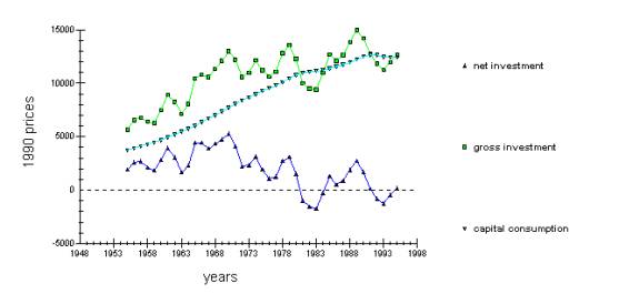
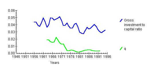
The investment in the UK has been highly volatile. Whereas gross investment has been rising steadily, the net investment has fallen from 1970-s onward. This is often associated with the productivity slowdown of western countries. However, from this graph it can be seen that increasingly, the resources go to depreciation. UK had also experienced the biggest recession since 1950-s a year before the net investment fell below zero, in 1979. This was partly attributed to the external oil-price shock. Thus, it might be that external supply shocks affect both income and investment and there is no direct link between them.
It can be that the UK has reached its optimal K/L ratio, as described by the Solow neo-classical growth model, but the Solow model takes technological change as given, which is surely not acceptable. However, the conventional measure of investment does not include expenditure on R&D, training and computers. It only describes the productive sector, not the service one. Thus, it might be that these sectors have become more important investment receivers. For example, it might be cheaper to produce given quantity by using the same amount of capital and more computers and more trained labour, than to increase the amount of capital.
Source: Summers, Robert and Heston, Alan, "The Penn World
Table (Mark 5.6): An expanded Set of International Comparisons,
1950-1988", Quarterly Journal Of Economics, vol 106, no. 9 (May 1991).
Its clear that UK invests less than either USA or Japan. It can be shown that UK also operates with considerably less capital per worker. Some writers have argued that this is the reason for lower GDP growth in the UK. However, investment is unimportant for the Solow growth model, thus it is hard to justify its association with growth rate in the neo-classical framework, but this model does not account for technological progress. Post neo-classical models (endogenous growth models etc.) emphasise the investment as a determinant of long-run growth.
I will now turn to empirical estimation of growth. Investment can be explained by scale and price variables. Early models normally ignored price variables (wage, profits, interest rates) and concentrated on scale (income). The implicit investment models take the lag structure of the model as given. In the simple fixed accelerator model (Clark 1917) investment only depends on the changes in output. Theoretically, when capital and labour are combined in a fixed proportion to produce output (clay-clay model) then as income increases, demand for products increases. To satisfy that demand firms will have to use more capital and thus invest more. However, it takes time for firms to build up capital stocks. Mayer (1958) has estimated from microeconomic data, that new plants take 21 months to build and new machinery takes about 7-8 months. In addition, financing arrangements are made normally just before the construction starts, about 15 months before completion. Still, Modigliani (1968) estimated that 60% of investment decisions are changed in response to new news about the economy. Thus, the investment can respond with a lag anywhere between 21-0 months. As I am using annualised data, this will mean that I will have to use approximately two lagged changes in income as an estimator for investment. Thus the microeconomic model of the investment is:
![]() (i)
(i)
NI – net investment, ut – random error (supply shocks, technology change).
I have data only for the index of manufacturing. I am converting that out of index form by using the fact that index=100 in 1990 when output=£116165m. Thus Y=indexY*116165/100. I am doing that transformation to enable me to calculate meaningful long-term response coefficients of net investment to changes in income. I will use the modelling technique based on Hendry et al., which, as Bean (1981) writes, "may be characterised as the intended over-parameterisation of models prior to data based simplification along lines suggested by some underlying economic theory". I will not use more than four lags due to degrees of freedom limitations, but I will include more lags than the microeconomic theory suggests, testing whether aggregation produces any significant problems.
Ordinary Least Squares Estimation for simple lagged accelerator model
*******************************************************************************
Dependent variable is NI
41 observations used for estimation from 1955 to 1995
*******************************************************************************
Regressor Coefficient Standard Error T-Ratio[Prob]
C 1035.3 256.9505 4.0291[.000]
DY .056242 .063450 .88640[.381]
DY(-1) .21211 .069748 3.0411[.004]
DY(-2) .18859 .071813 2.6261[.013]
DY(-3) .10757 .067059 1.6041[.118]
DY(-4) .064611 .061583 1.0492[.301]
*******************************************************************************
R-Squared .54724 R-Bar-Squared .48256
S.E. of Regression 1303.5 F-stat. F( 5, 35) 8.4606[.000]
Mean of Dependent Variable 1902.6 S.D. of Dependent Variable 1812.1
Residual Sum of Squares 5.95E+07 Equation Log-likelihood -349.0192
Akaike Info. Criterion -355.0192 Schwarz Bayesian Criterion -360.1599
DW-statistic .27547
DY= y-y(-1), y – IOP: D: Total manufacturing (IOM) £m. Blue book.
*******************************************************************************
* Test Statistics * LM version * F Version *
*******************************************************************************
* A:Serial Correlation*CHSQ( 1)= 31.0060[.000]*F( 1, 34)= 105.4831[.000]*
* B:Functional Form *CHSQ( 1)= .52509[.469]*F( 1, 34)= .44109[.511]*
* C:Normality *CHSQ( 2)= 1.4018[.496]* Not applicable *
* D:Heteroscedasticity*CHSQ( 1)= 4.9169[.027]*F( 1, 39)= 5.3143[.027]*
A:Lagrange multiplier test of residual serial correlation
B:Ramsey's RESET test using the square of the fitted values
C:Based on a test of skewness and kurtosis of residuals
D:Based on the regression of squared residuals on squared fitted values
Note: I will always use the same serial correlation, normality etc. tests.
I included further lags in the equation to determine whether aggregation has produced any anomalies. The coefficients for the first and second lags are significant, third lag becoming significant at 5% level when fourth lag is excluded. Immediate income is insignificant, roughly in accordance with Mayer’s predictions, and assuming investment is in some ways irreversible. Third lag is significant probably because firms will not have data available immediately.
However, there are problems with the serial correlation, suggesting that the dynamics is more complicated than that. Granger and Newbold have suggested that R2>DW is a good rule of thumb for spurious correlation. Net investment is probably generated by a difference stationary process. I will test whether investment series is time stationary, and if that causes serial correlation, and whether differencing it will eliminate the problem.
Unit root tests for variable NI
The Dickey-Fuller regressions include an intercept but not a trend
*******************************************************************************
38 observations used in the estimation of all ADF regressions.
Sample period from 1958 to 1995
*******************************************************************************
Test Statistic LL AIC SBC HQC
DF -1.7212 -317.3675 -319.3675 -321.0051 -319.9502
ADF(1) -2.7165 -313.3587 -316.3587 -318.8151 -317.2326
95% critical value for the augmented Dickey-Fuller statistic = -2.9400
Thus clearly test statistics are smaller than ADF critical value at 95% level, meaning that the hypotheses of non-stationarity cannot be rejected. Differentiating nid=ni-ni(-1)
Unit root tests for variable NID
Test Statistic LL AIC SBC HQC
DF -4.2765 -309.0046 -311.0046 -312.6155 -311.5725
ADF(1) -6.8668 -300.6561 -303.6561 -306.0724 -304.5080
95% critical value for the augmented Dickey-Fuller statistic = -2.9422
Now we can reject the hypotheses of non-stationarity. Thus one should include lagged investment to investment function – meaning that investment is either done of habit, or there are some slow moving variables affecting investment that I have not taken into account. The resulting formulation is what is called the dynamic accelerator model. Models like this are called ARDL(p,q) where p and q are the number of lags of DY and NI. To estimate p and q, I will first run regression with many lags and then do a variable deletion test.
Ordinary Least Squares Estimation
*******************************************************************************
Dependent variable is NI
39 observations used for estimation from 1957 to 1995
*******************************************************************************
Regressor Coefficient Standard Error T-Ratio[Prob]
C -30.4598 164.9973 -.18461[.855]
DY .10714 .031124 3.4423[.002]
DY(-1) .10713 .038570 2.7775[.009]
DY(-2) .010649 .041539 .25635[.799]
DY(-3) -.068840 .035590 -1.9343[.062]
NI(-1) 1.0593 .16794 6.3079[.000]
NI(-2) -.17811 .14833 -1.2007[.239]
Based on the fact that some of the coefficients are not significant at 5% level, I will test the exclusion of DY(-2), DY(-3) and NI(-2).
Variable Deletion Test (OLS case)
*******************************************************************************
Dependent variable is NI
List of the variables deleted from the regression:
DY(-2) DY(-3) NI(-2)
39 observations used for estimation from 1957 to 1995
*******************************************************************************
Regressor Coefficient Standard Error T-Ratio[Prob]
C -43.1376 162.2164 -.26593[.792]
DY .086075 .029939 2.8750[.007]
DY(-1) .16658 .029827 5.5850[.000]
NI(-1) .81711 .059593 13.7114[.000]
*******************************************************************************
Joint test of zero restrictions on the coefficients of deleted variables:
F Statistic F( 3, 32)= 2.0849[.122]
Thus, based on the p-value of F-test being more than 0.05, the restriction is not rejected at 5% level. The descriptive statistics of the restricted equation are:
R-Squared .88766 R-Bar-Squared .87830
S.E. of Regression 640.2377 F-stat. F( 3, 36) 94.8163[.000]
Mean of Dependent Variable 1902.1 S.D. of Dependent Variable 1835.2
Residual Sum of Squares 1.48E+07 Equation Log-likelihood -313.1239
Akaike Info. Criterion -317.1239 Schwarz Bayesian Criterion -320.5017
DW-statistic 1.6178 Durbin's h-statistic 1.3031[.193]
*******************************************************************************
Diagnostic Tests
* A:Serial Correlation*CHSQ( 1)= 1.4885[.222]*F( 1, 35)= 1.3527[.253]*
* B:Functional Form *CHSQ( 1)= .11390[.736]*F( 1, 35)= .099950[.754]*
* C:Normality *CHSQ( 2)= .13524[.935]* Not applicable *
* D:Heteroscedasticity*CHSQ( 1)= .030839[.861]*F( 1, 38)= .029319[.865]*
The model does not suffer from serial correlation or functional form problems.
As seen, the net investment series was generated by difference stationary process, similar to the process generating income. However, when regressing the difference of net investment against the difference in income one might miss valuable long-term information. Changes in income and net investment might be trending together stochastically, they might be co-integrated. To test for that, I will test the hypotheses that the DW d value=0 (CRDW test)
Dependent variable is NI
DW-statistic .42815
H0: there is cointegration; H1: there is not
Critical values for d: 0.511 at 1% level, 0.386 at 5% level
If computed DW<critical value, reject H0. In this case, we can reject H0 at 1% level, but not at 5% level. So it is not clear whether they are cointegrated or not. Thus it is not clear that the variables are cointegrated.
However, 1970-s was a period of supply shocks and the increase of inflationary expectations that might have changed the underlying relationship between changes in income and net investment. I testing for structural break in 1971-1974 and 1973 was the year that gave the highest F-test for the structural break:
* F:Chow Test *CHSQ( 2)= 32.1771[.000]*F( 2, 37)= 16.0885[.000]*
p-value of the F-test is 0, showing that there was very likely a structural break. From now on I will concentrate on the period after 1973.
Ordinary Least Squares Estimation
Dependent variable is NI
23 observations used for estimation from 1973 to 1995
Regressor Coefficient Standard Error T-Ratio[Prob]
DW-statistic .56297
One can not reject co-integration at 1% level. The long-run response of investment to output can be calculated by letting all the lagged values equal to their long-run values.
Based on OLS regression of NI on:
C DY(-1) DY(-2) NI(-1)
23 observations used for estimation from 1973 to 1995
*******************************************************************************
Coefficients A1 to A4 are assigned to the above regressors respectively
List of specified functional relationship(s):
longrun=(a2+a3)/(1-a4)
*******************************************************************************
Function Estimate Standard Error T-Ratio[Prob]
longrun .52577 .20460 2.5697[.017]
Thus the long-run response to a change in income will result in a change in net investment with half the magnitude. This suggests that capital accounts for half of the production, the other half being human capital and labour input increase.
To calculate the short-run effect of changes in income, one can look at the error correction mechanism. This assumes that adjustment to new levels of investment is costly and/or individuals will not realise the immediate effects when the income starts changing faster or slower. Thus the relationship is of the form:
In current case error = ni - 0.52577 * dy (the deviation from the long-term relationship)
Ordinary Least Squares Estimation
*******************************************************************************
Dependent variable is DNI
23 observations used for estimation from 1973 to 1995
*******************************************************************************
Regressor Coefficient Standard Error T-Ratio[Prob]
C 101.6225 143.3962 .70868[.487]
ERROR(-1) -.34524 .054796 -6.3003[.000]
DDY .051183 .029182 1.7540[.095]
*******************************************************************************
R-Squared .66557 R-Bar-Squared .63213
S.E. of Regression 672.5326 F-stat. F( 2, 20) 19.9018[.000]
Residual Sum of Squares 9046001 Equation Log-likelihood -180.7825
DW-statistic 1.3859
* A:Serial Correlation*CHSQ( 1)= 2.6827[.101]*F( 1, 19)= 2.5087[.130]*
* B:Functional Form *CHSQ( 1)= .012438[.911]*F( 1, 19)= .010280[.920]*
* C:Normality *CHSQ( 2)= .93003[.628]* Not applicable *
* D:Heteroscedasticity*CHSQ( 1)= 1.0077[.315]*F( 1, 21)= .96224[.338]*
As seen, the error correction mechanism describes the data rather well. 35% of the error in overestimating the change in income the period before is corrected the next period.
Similar to the error correction mechanism is the mechanism with quadratic adjustment costs. It assumes that the costs of investment get larger, as investment increases. It is further assumed that desired capital stock is a proportion of output, and that each period part of the discrepancy is eliminated by investment (but not all, because it is cheaper to adjust the capital stock in several periods). Otherwise the output is similar to the dynamic accelerator model.
The reason for including lNKt-1 is that statistics refer to investment at the end of the period. The reason for using Yt-1 is that when firms decide how much to invest in period t, they will not know what Yt will be, so the simplest assumption is to say that they will predict Y to remain the same.
Ordinary Least Squares Estimation
*******************************************************************************
Dependent variable is NI
22 observations used for estimation from 1972 to 1993
*******************************************************************************
Regressor Coefficient Standard Error T-Ratio[Prob]
C -12665.9 3039.9 -4.1665[.001]
Y(-1) .14921 .030707 4.8591[.000]
NK(-1) -6.7279 1.3682 -4.9174[.000]
*******************************************************************************
R-Squared .63890 R-Bar-Squared .60089
S.E. of Regression 972.6107 F-stat. F( 2, 19) 16.8087[.000]
Mean of Dependent Variable 996.7612 S.D. of Dependent Variable 1539.5
Residual Sum of Squares 1.80E+07 Equation Log-likelihood -180.9637
Akaike Info. Criterion -183.9637 Schwarz Bayesian Criterion -185.6002
DW-statistic .75864
*******************************************************************************
Diagnostic Tests
*******************************************************************************
* Test Statistics * LM version * F Version *
*******************************************************************************
* A:Serial Correlation*CHSQ( 1)= 9.6872[.002]*F( 1, 18)= 14.1616[.001]*
* B:Functional Form *CHSQ( 1)= 1.9628[.161]*F( 1, 18)= 1.7632[.201]*
* C:Normality *CHSQ( 2)= 1.6413[.440]* Not applicable *
* D:Heteroscedasticity*CHSQ( 1)= 2.4021[.121]*F( 1, 20)= 2.4514[.133]*
Again, this model does well, in terms of showing that net capital is important. It is the basis of much frequently used and theoretically more sound Neoclassical model.
Neoclassical
model.
Despite the good description that these models give to data, they lack cost of capital variables from the right-hand side. Jorgenson’s (1963) theory of investment intended to remedy this situation. Assuming no adjustment costs, and Cobb-Douglas production, and constant returns to scale, then Jorgenson obtained the standard first order condition:
K=aY/Ck, where Ck is the cost of capital and a is the share of capital in a standard Cobb-Douglas production function. This model had also problems with serial correlation and due to space limitation, I will not replicate it. It gave way to the flexible neoclassical model of Hall and Jorgenson, where the desired level of capital, K* was used instead of K. Ckt=pt(rt+dt)(1-tt) where p is the price of capital, r is the interest rate, d is the depreciation and t is the tax rate on business income. The effects of capital appreciation are also likely to reduce the costs of new capital.
Summers, Robert and Heston, Alan, "The Penn World Table
(Mark 5.6): An expanded Set of International Comparisons, 1950-1988",
Quarterly Journal Of Economics, vol 106, no. 9 (May 1991)
Dependent variable is LI
22 observations used for estimation from 1972 to 1993
*******************************************************************************
Regressor Coefficient Standard Error T-Ratio[Prob]
C 2.0131 .67451 2.9846[.009]
RK(-1) -.1196E-5 .9618E-6 -1.2436[.233]
RK(-2) -.2358E-5 .1075E-5 -2.1938[.044]
LWAGE(-1) -.40246 .063655 -6.3226[.000]
LPROFIT .40940 .050780 8.0621[.000]
LI(-1) .25563 .10984 2.3274[.034]
LY(-1) .57296 .16978 3.3747[.004]
*******************************************************************************
R-Squared .93829 R-Bar-Squared .91361
S.E. of Regression .036901 F-stat. F( 6, 15) 38.0151[.000]
Mean of Dependent Variable 9.3761 S.D. of Dependent Variable .12555
Residual Sum of Squares .020425 Equation Log-likelihood 45.5858
Akaike Info. Criterion 38.5858 Schwarz Bayesian Criterion 34.7672
DW-statistic 2.0569 Durbin's h-statistic -.15577[.876]
*******************************************************************************
* A:Serial Correlation*CHSQ( 1)= .11566[.734]*F( 1, 14)= .073989[.790]*
* B:Functional Form *CHSQ( 1)= .0082176[.928]*F( 1, 14)= .0052313[.943]*
* C:Normality *CHSQ( 2)= 1.3216[.516]* Not applicable *
* D:Heteroscedasticity*CHSQ( 1)= .55339[.457]*F( 1, 20)= .51606[.481]*
None of the models discussed before considered expectations of future profits when calculating the optimal capital. In this section I will look at the q – theory of investment, that uses the future information available through the stock markets. However, as will be shown, the q-theory will not fit data very well, mostly because of the uncertainties, risk aversion and imperfect capital markets due to asymmetric information. Thus, the models I deal with have to make numerous very simplifying assumptions. Still, these models are theoretically sound and good basis for future work. Implicit models are not very well suited for forecasting, as they suffer from the Lucas Critique – as they do not use the expectation variables, once they are published and the expectations change, the models are of very limited use.
Q
theory.
First explicit model was the Brainard and Tobin’s (1968) q theory. They argued that “investment should be an increasing function of the ratio of the value of the firm to the cost of purchasing the firm’s equipment and structures in their respective markets.” Cabalero(1997). This ratio, the average q, summarises most of the information about future actions and shocks that the firm might experience. I=γq, γ>0.
Abel and Hayashi (1982) showed that the neoclassical model yields a marginal value of q. Marginal and average q are equal in perfect competition or when production function and adjustment costs are linearly homogeneous. This is an important point, because marginal q is unobservable (it is the shadow price of capital), but the average q is (it is the existing price of capital relative to present stock market value).
Here, I am considering a very simple q model by Hassert and Huban (NBER 5683 1996). Assume that firms are price takers. Absent of taxes, firms real net cash flow is:
![]()
where K(.) is the capital stock, F(.) is the real revenue
function, N is the variable factor (like Labour), w is its price, p is price of
investment goods and C(.) is the function determining the cost of adjustment.
Firm maximises the present value of its future cash flow:
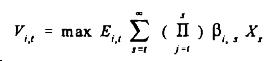
where E is the expectations operator for firm i, conditional
to the information available at time t, and b is the discount factor for the
firm. In equilibrium, the shadow value of additional unit of investment, q
equals its marginal cost.
q=pt+Ct
Δq=rq+FK+CK where r is instantaneous discount rate.
If we assume that the adjustment costs are quadratic:
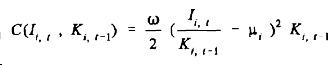
where μ is the steady state rate of investment and ω
is the adjustment cost parameter, then the firms profit maximising condition
can be expressed as:

This is a convenient way of estimating the investment changes
to neoclassical variables of price etc. However, marginal q here is
unobservable. Approximating average q (denoted by Q) for marginal q yields:
where V is the market value of firms equity, B is the market
value of firms debt and K is the replacement value of firm’s capital stock.
Because the model is derived directly from optimisation, it is theoretically
sound, recognises the dynamics of technology and expectations and isolates
their effects. The value of the capital stock=price*quantity. Thus, it is
approximately the current price level of capital goods times the gross capital
on aggregate. Multiplying through by capital stock yields:
The above mentioned equation is difficult to estimate. I will first run a regression without the cost of capital, denoting It/Kt-1 as GiGK1, gross investment over gross capital. pt-1 is the price index of capital goods, Kt-i is the net value of capital and Vt is the Financial Times stock market index.
Ordinary Least Squares Estimation
*******************************************************************************
Dependent variable is GIGK1
21 observations used for estimation from 1972 to 1992
*******************************************************************************
Regressor Coefficient Standard Error T-Ratio[Prob]
C .032470 .0016059 20.2191[.000]
FTNKPI(-1) .70145 .28695 2.4445[.024]
*******************************************************************************
R-Squared .23926 R-Bar-Squared .19922
S.E. of Regression .0039649 F-stat. F( 1, 19) 5.9756[.024]
Mean of Dependent Variable .035777 S.D. of Dependent Variable .0044308
Residual Sum of Squares .2987E-3 Equation Log-likelihood 87.3887
Akaike Info. Criterion 85.3887 Schwarz Bayesian Criterion 84.3442
DW-statistic .79006
*******************************************************************************
* A:Serial Correlation*CHSQ( 1)= 7.3705[.007]*F( 1, 18)= 9.7339[.006]*
* B:Functional Form *CHSQ( 1)= 6.1462[.013]*F( 1, 18)= 7.4480[.014]*
* C:Normality
*CHSQ( 2)= .64941[.723]* Not applicable
*
* D:Heteroscedasticity*CHSQ( 1)= 1.5156[.218]*F( 1, 19)= 1.4779[.239]*
As seen the measure of q (FTNKPI(-1) is significant at 5% level, although the regression suffers from serial correlation and has low R2 value.
Now I run the regression with the cost of capital measures present:
Ordinary Least Squares Estimation
*******************************************************************************
Dependent variable is GIGK1
21 observations used for estimation from 1972 to 1992
*******************************************************************************
Regressor Coefficient Standard Error T-Ratio[Prob]
C .013578 .0047798 2.8408[.012]
FTNKPI(-1) -.38458 .29755 -1.2925[.215]
DWAGES(-1) -.8329E-3 .2070E-3 -4.0228[.001]
R(-1) -.4187E-4 .2551E-3 -.16413[.872]
GIGK1(-1) .78933 .14868 5.3087[.000]
*******************************************************************************
R-Squared .75272 R-Bar-Squared .69091
S.E. of Regression .0024633 F-stat. F( 4, 16) 12.1763[.000]
Mean of Dependent Variable .035777 S.D. of Dependent Variable .0044308
Residual Sum of Squares .9709E-4 Equation Log-likelihood 99.1885
Akaike Info. Criterion 94.1885 Schwarz Bayesian Criterion 91.5772
DW-statistic 1.7193 Durbin's h-statistic .87871[.380]
* Test Statistics * LM Version * F Version *
*******************************************************************************
* A:Serial Correlation*CHSQ( 1)= .074582[.785]*F( 1, 15)= .053463[.820]*
* B:Functional Form *CHSQ( 1)= 7.6924[.006]*F( 1, 15)= 8.6706[.010]*
* C:Normality *CHSQ( 2)= .16363[.921]* Not applicable *
* D:Heteroscedasticity*CHSQ( 1)= 3.9304[.047]*F( 1, 19)= 4.3749[.050]*
To test which model suits the data best, I could look at the N test for testing non-nested models. In this model H0: original model is true, H1 alternative model is true. Then original and alternative models are swapped and the test is repeated. The test is decisive, when H0 is rejected in one case, and accepted in another. However, due to space limitations I will not. It is clear that the quantity models perform better (ARDL model) than cost models (Neoclassical) and models with explicit lags (q-theory). However, modern q-theory has developed significantly, and it has the advantage theoretically sound predictions to the future.
For the long-term relationship, it is clear that the net investment is now less than 20 years ago. The models explain it by the slowing down of income growth, probably because productivity has fallen. In addition, it looks like the depreciation is now so high that it crowds out net investment. However, it might be the low investment instead that causes slow income growth. The low investment might be due to statistical reasons. 1970-s with its oil-price shock might have initiated a long structural change in economy towards information technology and services. Existing capital must depreciate, however, not all of the new capital is counted (the quality of the computers is not counted). There might have also been changes in the corporate tax system. income taxes have been reduced, so firms will have a greater incentive to pay wages and invest less. Q theory also shows that the market valuation of firms has fallen. This is due to markets getting very sophisticated and international, one cannot just float anything on the stockmarket anymore. In addition, it might be that investors have started only to concentrate on the short-term gains. Foreign direct investment (i.e. by Japanese car manufactures to enter the EU market) might have crowded out the manufacturing investment. This can be seen by the generally increased interest rates for investment.
Short-term fluctuations are most likely caused by income fluctuations. Real Business Cycle and New Keynesian nominal friction fluctuation models each provide a different theoretical route to that result. RBC models assume that technology shocks happen occasionally, and because of special propagation mechanisms, investment is more volatile. New Keynesians model how the small microeconomic nominal frictions will lead to large frictions on aggregate (menu costs).
Finally,
government has created much of the changes. Privatisation probably adds to the
change in long-term structure, whereas the experiments with interest rates and
monetary policy have caused short-term fluctuations (RBC models can explain those
findings elegantly).
Due to the
many factors affecting it, investment is very hard to model empirically based
on theoretical reasoning. Most of the models can only explain the investment
changes ad hoc.
Bean “An Econometric Model of the manufacturing Investment in the UK”. Economic Journal, March 1981
Caballero “Aggregate Investment”, NBER working paper 6264
Chirinko “Business Fixed Investment Spending” Journal of Economic Literature 1993 dec.
Driver and Moreton “The Influence of Uncertainty on UK Manufacturing Investment”. Economic Journal November 1991
Hassett, Hubbard NBER working paper 5683 “Tax Policy and Investment”.
Nickell “The
investment decisions of firms”
Peterson “Fixed
Investment” 1987
Romer “Advanced
Macroeconomics”
Data sources
are generally from the faculty network, unless otherwise stated.
The list of variables used:
R - Treasury
bills: average discount rate
PROFIT All cos
(ICCs + FCs): Gross trading profits (inc. stock appreciation) #m NSA
EXEGAU Gross
capital stock: manufacturing (revised definition)(1990 prices) #bn
GK exegau*1000
FT FT:
ordinary industrial share index (1935=100)
LY log(y )
Y IOP: D:
Total manufacturing (IOM) (1990)*116165/100